Unveiling the Power of Quantization

Introduction

Let’s say you have a talented friend who can recognize patterns, like determining whether an image contains a cat or a dog. Now, this friend has a precise way of doing things, like he has a dictionary in his head. But, here’s the problem: this encyclopedia is huge and requires significant time and effort to use.

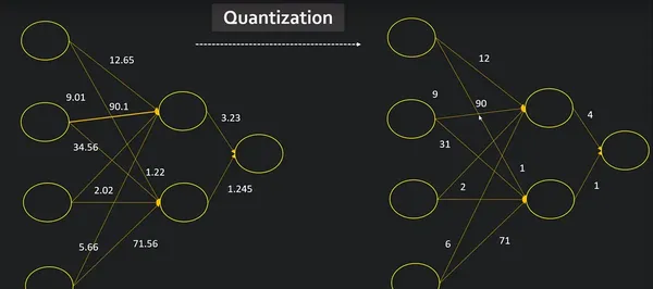
Consider simplifying the process, like converting that big encyclopedia into a convenient cheat sheet. This is similar to the way model quantization works for clever computer programs. It takes these intelligent programs, which can be excessively large and sluggish, and streamlines them, making them faster and less demanding on the machine. How does this work? Well, it’s similar to rounding off difficult figures. If the numbers in your friend’s encyclopedia were really extensive and comprehensive, you can decide to simplify them to speed up the process. Model quantization techniques, reduce the ‘numbers’ that the computer uses to recognize objects.

So why should we care? Imagine that your friend is helping you on your smartphone. You want it to be able to recognize objects fast without taking up too much battery or space. Model quantization makes your phone’s brain operate more effectively, similar to a clever friend who can quickly identify things without having to consult a large encyclopedia every time.

Learning Objectives

• Examine key components of quantization, encompassing weights and activations in a neural network.
• Explore various techniques for model quantization to optimize efficiency and reduce memory usage.
• Understand how quantization impacts a simple neural network by analyzing its architecture and performance.
• Compare the size and performance of a quantized convolutional neural network against its original counterpart.

This article was published as a part of the Data Science Blogathon.

What is Model Quantization?

Quantization is a method that can allow models to run faster and use less memory. By converting 32-bit floating-point numbers (float32 data type) to lower-precision formats such as 8-bit integers (int8 data type), we can reduce the computational requirements of our model.

Quantization is the process of reducing the precision of a model’s weights and activations from floating-point to smaller bit-width representations. It aims to increase the adaptability of the model for deployment on constrained devices such as smartphones and embedded systems by reducing memory footprint and increasing inference speed.

Why Do We Need Model Quantization?

Model quantization is essential for many reasons, especially when deploying machine learning models in real-world scenarios. Here are the major reasons for the need for model quantization:

• Limited Memory Resources: Resource-constrained devices, such as mobile phones, IoT devices, and edge computing devices, often have limited memory. Quantization significantly reduces the memory footprint of models, making them more feasible to deploy on such devices.
• Lower Energy Consumption: Quantized models typically require less computation, leading to lower energy consumption during both training and inference. This is especially important for battery-powered devices and environments where energy efficiency is a priority.
• Faster Inference: Quantization reduces the precision of weights and activations, resulting in fewer arithmetic operations during inference. This results in faster model execution, which is important for real-time applications and services that require quick responses.

What Are The Key Aspects Of Model Quantization?

Model quantization is a technique used in machine learning to reduce the memory requirements and computational cost of a trained model. The goal is to make models more efficient, especially for deployment on resource-constrained devices such as mobile phones, embedded systems or edge devices. This process involves representing the parameters (weights and activations) of the model using a reduced number of bits.

Here are the key aspects of model quantization:

1. Parameter Quantization

This involves reducing the accuracy of the model’s weights. Typically, deep learning models use 32-bit floating-point numbers to represent weights. In quantization, these values are replaced with lower-bit representations, such as 8-bit integers. This reduces the memory footprint of the model and speeds up inference.

2. Activation Quantization

In addition to quantizing the weights, quantization can be applied to the activation values produced by each layer during inference. Activation quantization involves representing intermediate feature maps with lower-precision data types, further reducing memory requirements.

3. Post-training and Quantization-aware Training

Model quantization can be performed after a model has been trained (quantization after training) or during the training process (quantization-aware training). Quantization-aware training involves adjusting the training process to take into account low accuracy during forward and backward passes.

4. Dynamic Quantization

In dynamic quantization, the accuracy of the model’s weights is dynamically optimized during inference based on the observed range of activation values. This allows greater flexibility and can improve model performance.

Benefits of Model Quantization

The benefits of model quantization include:

• Low Model Size: Quantized models have a small memory footprint, making them suitable for deployment on devices with limited storage.
• Faster estimation: Low-precision calculations require fewer computational resources, resulting in faster estimation times. This is especially important for real-time applications.
• Energy Efficiency: Lower computational requirements also result in lower energy consumption, which is important for devices with limited battery life.

Despite these advantages, the model comes with quantification challenges. Lower precision can lead to a loss of model accuracy, and finding the right balance between model size, inference speed, and accuracy is often a trade-off. Achieving optimal results for a specific use case requires careful consideration and sometimes fine-tuning.

Model Quantization

Post-training quantization includes general techniques to reduce CPU and hardware accelerator latency, processing, power, and model size with little degradation in model accuracy. These techniques can be performed on an already-trained float TensorFlow model and applied during TensorFlow Lite conversion.

import tensorflow as tf
from tensorflow import keras
import numpy as np
import pathlib  

Training The Model

mnist = keras.datasets.mnist
(train_images, train_labels), (test_images, test_labels) = mnist.load_data()

# Normalize the input image so that each pixel value is between 0 to 1.
train_images = (train_images / 255.0).astype(np.float32)
test_images = (test_images / 255.0).astype(np.float32)

# Define the model architecture
model = keras.Sequential([
  keras.layers.InputLayer(input_shape=(28, 28)),
  keras.layers.Reshape(target_shape=(28, 28, 1)),
  keras.layers.Conv2D(filters=12, kernel_size=(3, 3), activation=tf.nn.relu),
  keras.layers.MaxPooling2D(pool_size=(2, 2)),
  keras.layers.Flatten(),
  keras.layers.Dense(10)
])

# Train the digit classification model
model.compile(optimizer="adam",
              loss=keras.losses.SparseCategoricalCrossentropy(from_logits=True),
              metrics=['accuracy'])
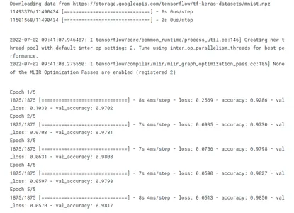
model.fit(
  train_images,
  train_labels,
  epochs=5,
  validation_data=(test_images, test_labels)
)

models_dir = pathlib.Path('models')
models_dir.mkdir(exist_ok=True, parents=True)
model.save(f'{models_dir}/tf_model.h5')

Various Quantization Techniques

Quantization is a process used in digital signal processing and data compression to reduce the number of bits needed to represent data without losing too much information. In the context of machine learning and neural networks, quantization is often employed to reduce the precision of weights and activations, leading to more efficient model deployment on hardware with limited resources. Here are some various quantization techniques:

1. Convert to a TensorFlow Lite Model

TensorFlow Lite converts weights to 8-bit precision as part of the model conversion from TensorFlow graphdefs to TensorFlow Lite’s flat buffer format.

converters = tf.lite.TFLiteConverter.from_keras_model(model)
tflite_models = converters.convert()
tflite_model_files = models_dir/"tflite_model.tflite"
tflite_model_files.write_bytes(tflite_models)

2. Dynamic Quantization

The simplest form of post-training quantization techniques statically quantizes only the weights from floating point to integer, which has 8 bits of precision. At inference, weights are converted from 8-bits of precision to
floating point and computed using floating-point kernels. This conversion is done once and cached to reduce latency.

converter = tf.lite.TFLiteConverter.from_keras_model(model)
converter.optimizations = [tf.lite.Optimize.DEFAULT]
tflite_dynamic_quant_model = converter.convert()
tflite_dynamic_quant_model_file = models_dir/"tflite_dynamic_quant_model.tflite"
tflite_dynamic_quant_model_file.write_bytes(tflite_dynamic_quant_model)

3. Integer Quantization

Integer quantization is an optimization strategy that converts 32-bit floating-point numbers (such as weights and activation outputs) to the nearest 8-bit fixed-point numbers. This results in a smaller model and increased inferencing speed.

To quantize the variable data (such as model input/output and intermediates between layers), you need to provide a Representative Dataset. This is a generator function that provides a set of input data that’s large enough to represent typical values. It allows the converter to estimate a dynamic range for all the variable data. (The dataset does not need to be unique compared to the training or evaluation dataset.)

To support multiple inputs, each representative data point is a list, and elements in the list are fed to the model according to their indices.

def representative_data_gen():
    for input_value in tf.data.Dataset.from_tensor_slices(train_images).batch(1).take(100):
        yield [input_value]

converter = tf.lite.TFLiteConverter.from_keras_model(model)
converter.optimizations = [tf.lite.Optimize.DEFAULT]
converter.representative_dataset = representative_data_gen
# Ensure that if any ops can't be quantized, the converter throws an error
converter.target_spec.supported_ops = [tf.lite.OpsSet.TFLITE_BUILTINS_INT8]
# Set the input and output tensors to uint8 
converter.inference_input_type = tf.uint8
converter.inference_output_type = tf.uint8

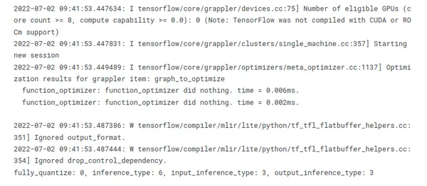
tflite_int_quant_model = converter.convert()
tflite_int_quant_model_file = models_dir/"tflite_int_quant_model.tflite"
tflite_int_quant_model_file.write_bytes(tflite_dynamic_quant_model)

4. Float 16 Quantization

Converting weights to 16-bit floating point values during model conversion from TensorFlow to TensorFlow Lite’s flat buffer format, results in a 2x reduction in model size. Some hardware, like GPUs, can
compute natively in this reduced precision arithmetic, realizing a speedup over traditional floating point execution. The Tensorflow Lite GPU delegate can be configured to run in this way.

However, a model converted to float16 weights can still run on the CPU without additional modification: the float16 weights are upsampled to float32 prior to the first inference. This permits a significant reduction in model size in exchange for a minimal impact on latency and accuracy.

converter = tf.lite.TFLiteConverter.from_keras_model(model)
converter.optimizations = [tf.lite.Optimize.DEFAULT]
converter.target_spec.supported_types = [tf.float16]
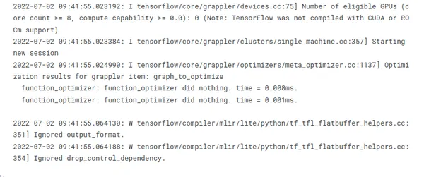
tflite_float16_quant_model = converter.convert()
tflite_float16_quant_model_file = models_dir/"tflite_float16_quant_model.tflite"
tflite_float16_quant_model_file.write_bytes(tflite_float16_quant_model)

5. 16×8 Quantization

Converting activations to 16-bit integer values and weights to 8-bit integer values during model conversion from TensorFlow to TensorFlow Lite’s flat buffer format can improve the accuracy of the quantized model significantly, when activations are sensitive to the quantization, while still achieving almost 3-4x reduction in model size. Moreover, this fully quantized model can be consumed by integer-only hardware accelerators.

converter = tf.lite.TFLiteConverter.from_keras_model(model)
converter.optimizations = [tf.lite.Optimize.DEFAULT]
converter.target_spec.supported_ops = [tf.lite.OpsSet.
    EXPERIMENTAL_TFLITE_BUILTINS_ACTIVATIONS_INT16_WEIGHTS_INT8]
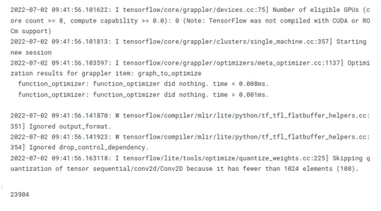
tflite_16x8_quant_model = converter.convert()
tflite_16x8_quant_model_file = models_dir/"tflite_16x8_quant_model.tflite"
tflite_16x8_quant_model_file.write_bytes(tflite_16x8_quant_model)

How Does Quantization of a Simple Neural Network Work?

Let’s apply quantization to a neural network. We’ll create a simple network with one hidden layer, then we’ll quantize and dequantize its weights.

In PyTorch, quantization is achieved using a QuantStub and DeQuantStub to mark the points in the model where the data needs to be converted to quantized form and converted back to floating point form, respectively. After defining the network with these stubs, we use the torch.quantization.prepare and torch.quantization.convert functions to quantize the model.

The process of quantizing a model in PyTorch involves the following steps:

• Define a neural network and mark the points in the model where the data needs to be converted to quantized form and converted back to floating point form. This is done using a quantization-aware training approach, where specific layers or operations are identified for quantization.
• Specify a quantization configuration for the model using torch.quantization.QConfig. This configuration defines how the model should be quantized, including precision settings and target devices.
• Prepare the model for quantization using torch.quantization.prepare. This step involves setting the model to the training mode and inserting fake quantization modules to simulate quantization during training.
• Calibrate the model on a calibration dataset. During calibration, the model is run on a calibration dataset, and the range of the activations is observed. This is used to determine the parameters for quantization, ensuring an accurate representation of the data.
• Convert the prepared and calibrated model to a quantized version using torch.quantization.convert. This function changes these modules to use quantized weights, completing the process and producing a quantized version of the original neural network.

Import all necessary libraries:

import numpy as np
import matplotlib.pyplot as plt
import torch
import torch.nn as nn
import torch.optim as optim
import torchvision
import torchvision.transforms as transforms
from torch.utils.data import DataLoader
import sys
import io

# Define the network architecture
class Net(nn.Module):
    def __init__(self):
        super(Net, self).__init__()

        self.quant = torch.quantization.QuantStub()
        

        self.fc1 = nn.Linear(28 * 28, 128)  
        self.fc2 = nn.Linear(128, 10) 


        self.dequant = torch.quantization.DeQuantStub()

    def forward(self, x):
        # Reshape the input tensor to a vector of size 28*28
        x = x.view(-1, 28 * 28)
        

        x = self.quant(x)
        

        x = torch.relu(self.fc1(x))
        
        # Apply the second fully connected layer
        x = self.fc2(x)
        

        x = self.dequant(x)
        
        return x

# Load the MNIST dataset
transform = transforms.Compose([transforms.ToTensor(), transforms.Normalize
            ((0.1307,), (0.3081,))])
trainset = torchvision.datasets.MNIST(root="../working/cache", train=True,
               download=True, transform=transform)
trainloader = DataLoader(trainset, batch_size=64, shuffle=True)

# Define loss function and optimizer
net = Net()
criterion = nn.CrossEntropyLoss()
optimizer = optim.SGD(net.parameters(), lr=0.01)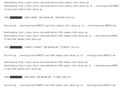

# Train the network
for epoch in range(2):  # loop over the dataset multiple times
    running_loss = 0.0
    for i, data in enumerate(trainloader, 0):
        # get the inputs; data is a list of [inputs, labels]
        inputs, labels = data

        # zero the parameter gradients
        optimizer.zero_grad()

        # forward + backward + optimize
        outputs = net(inputs)
        loss = criterion(outputs, labels)
        loss.backward()
        optimizer.step()

        # print statistics
        running_loss += loss.item()
        if i % 200 == 199:    # print every 200 mini-batches
            print("[%d, %5d] loss: %.3f" %
                  (epoch + 1, i + 1, running_loss / 200))
            running_loss = 0.0

print("Finished Training")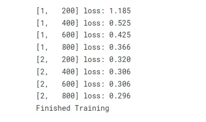

# Specify quantization configuration
net.qconfig = torch.ao.quantization.get_default_qconfig("onednn")

# Prepare the model for static quantization.

net_prepared = torch.quantization.prepare(net)

# Now we convert the model to a quantized version.
net_quantized = torch.quantization.convert(net_prepared)


buf = io.BytesIO()
torch.save(net.state_dict(), buf)
size_original = sys.getsizeof(buf.getvalue())

buf = io.BytesIO()
torch.save(net_quantized.state_dict(), buf)
size_quantized = sys.getsizeof(buf.getvalue())

print("Size of the original model: ", size_original)
print("Size of the quantized model: ", size_quantized)
print(f"The quantized model is {np.round(100.*(size_quantized )/size_original)}% the size of the original model")

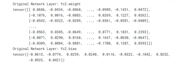
# Print out the weights of the original network
for name, param in net.named_parameters():
    print("Original Network Layer:", name)
    print(param.data)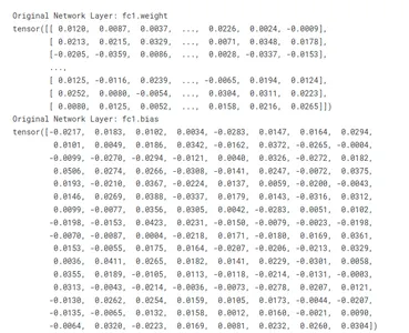

# Print out the weights of the quantized network
for name, module in net_quantized.named_modules():
    if isinstance(module, nn.quantized.Linear):
        print("Quantized Network Layer:", name)
        
        print("Weight:")
        print(module.weight())
        
        print("Bias:")
        print(module.bias)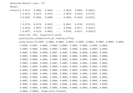

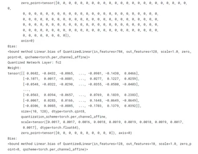
Comparing a Quantized and Non-Quantized Model

The below example shows how the quantized model can be used in the same way as the original model. It also demonstrates the trade-off between precision and memory usage/computation speed that comes with quantization. The quantized model uses less memory and is faster to compute, but the outputs are not the same as the original model due to the quantization error.

Here is a summary of the details and a comparison with the original model:

• Tensor Values: In the quantized model, these are quantized values of the weights and biases, compared to the original model which stores these in floating point precision. These values are
  used in the computations performed by the layer, and they directly affect the layer’s output.
• Size: This is the shape of the weight or bias tensor and it should be the same in both the original and quantized model. In a fully connected layer, which corresponds to the number of neurons in the current layer and the number of neurons in the previous layer.
• Dtype: In the original model, the data type of the tensor values is usually torch.float32 (32-bit floating point), whereas in the quantized model, it is a quantized data type like torch.qint8 (8-bit quantized integer). This reduces the memory usage and computational requirements of the model.
• Quantization_scheme: This is specific to the quantized model. It is the type of quantization used, for example, torch.per_channel_affine means different channels (e.g., neurons in a layer) can have a different scale and zero_point values.
• Scale & Zero Point: These are parameters of the quantization process and are specific to the quantized model. They are used to convert between the quantized and dequantized forms of the
  tensor values.
• Axis: This indicates the dimension along which the quantization parameters vary. This is also specific to the quantized model.
• Requires_grad: This indicates whether the tensor is a model parameter that is updated during training. It should be the same in both the original and quantized models.

# Suppose we have some input data
input_data = torch.randn(1, 28 * 28)

# We can pass this data through both the original and quantized models
output_original = net(input_data)
output_quantized = net_quantized(input_data)

# The outputs should be similar, because the quantized model is a lower-precision
# approximation of the original model. However, they won't be exactly the same
# because of the quantization process.
print("Output from original model:", output_original.data)
print("Output from quantized model:", output_quantized.data)

# The difference between the outputs is an indication of the "quantization error",
# which is the error introduced by the quantization process.
quantization_error = (output_original - output_quantized).abs().mean()
print("Quantization error:", quantization_error)

# The weights of the original model are stored in floating point precision, so they
# take up more memory than the quantized weights. We can check this using the
# `element_size` method, which returns the size in bytes of one element of the tensor.
print(f"Size of one weight in original model: {net.fc1.weight.element_size()} bytes (32bit)")
print(f"Size of one weight in quantized model: {net_quantized.fc1.weight().element_size()} byte (8bit)")

Conclusion

Model quantization is the process of making smart programs on our computers more compact and quicker, allowing them to function properly even on smaller machines. It’s like transforming your computer’s brain into a faster, more efficient assistant!

As the field of machine learning continues to evolve, the effective use of quantization techniques remains crucial for enabling the deployment of efficient and high-performance models across a variety of platforms, from edge devices to resource-constrained environments.

Key Takeaways

• Quantization techniques can be used to reduce the precision of deep learning models and improve their efficiency.
• There are several approaches to quantization, including post-training quantization and quantization-aware training.
• Best practices for quantization include choosing the appropriate precision, using a representative dataset, fine-tuning the model, and monitoring the accuracy.
• The balance between accuracy and efficiency will depend on the specific characteristics of the model and the task at hand.

Frequently Asked Questions

The media shown in this article is not owned by Analytics Vidhya and is used at the Author’s discretion.